Hlookup In Excel 2016 Between Multiple Worksheets

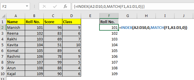
In Excel the mixed INDEXT and MATCH function is powerful for us to vlookup values based on one or more criteria to know this formula do as follows. Notice the only difference between the two formulas is the the row index.

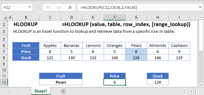
How To Use Vlookup And Hlookup Functions In Excel 2016 Dummies

Adding Text.

Hlookup in excel 2016 between multiple worksheets. Use VLOOKUP when your comparison values are located in a column to the left of the data you want to find. This converts the data to an Excel data table. Aligning Cell Content TUTORIAL - Excel 2016.

HLOOKUP C5 table21 get level. This approach involves converting all the data in the Division tabs into Excel data tables. Press CTRL T to display the Create Table window.

You could do something like this IFISERRRORHLOOKUPA1B1Z1003FALSEHLOOKUPA1SHEET2B1Z1003FALSEHLOOKUPA1B1Z1003FALSE. Adding Text. For more on using HLOOKUP across multiple documents watch this.

HLOOKUP C5 table31 get bonus. Although the Excel lookup functions can seem quite straightforward its very easy to get the wrong answer if you dont fully understand how they work. Ill choose first example here to dissect and ensure that you understand the basic use of the function.

Select a blank cell you want to place the summing result enter this formula SUMPRODUCTHLOOKUPB15A1M12234567891011120 and press Enter key now you get the summing result. Vlookup value with multiple criteria with INDEXT and MATCH function. Data Entry Formatting - Excel 2016 5 TUTORIALS 5 TESTS.

The H in HLOOKUP stands for Horizontal. Click on any data cell in the Division tab. HLOOKUP from another workbook or worksheet.

A generic formula to Vlookup across sheets is as follows. For example lets say you want to perform an HLOOKUP on the current sheet and if that fails perform an HLOOKUP on a second sheet. To get Bonus the formula in E5 copied down is.

In general h-lookup from another sheet or a different workbook means nothing else than supplying external references to your HLOOKUP formula. Here I introduce some formulas to help you quickly sum a range of values based on a value. Youll see how the index parameter value affects the outcome.

Then we will drag it to the remaining cells. It means giving an external reference to our HLOOKUP formula. Use of HLOOKUP to return multiple values from a single Horizontal LOOKUP.

Next Excel will process your VLOOKUP formula. Moving vertically down the left side of the table array selected red border table stop at the lookup value Brazil and return the value in the corresponding fourth column result of HLOOKUP 4 The resulting value for the entire formula combination is 85578. One more way to Vlookup between multiple sheets in Excel is to use a combination of VLOOKUP and INDIRECT functions.

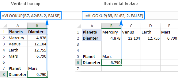
Speaking in a technical way the generic definition of the VLOOKUP function is that it looks up for a value in the first column of the specified range and returns a similar value in the same row from another column. For each amount in C5C13 the goal is to find the best match not an exact match. To lookup Level the formula in cell D5 copied down is.

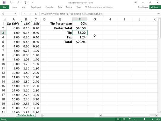
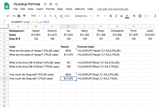
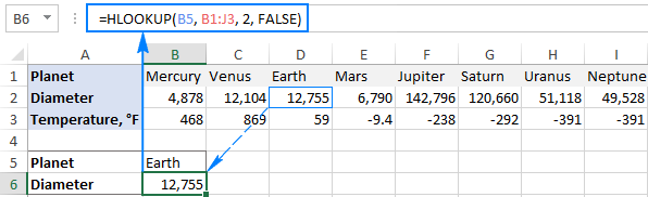
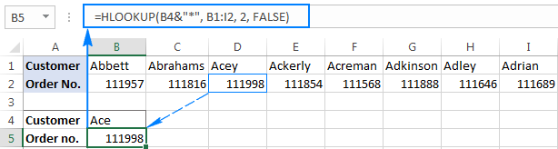
The formula Hlookup 11876B1K32False is used to tell the function to search for the value 11876 within the range of. Excel does have an additional lookup function. DOWNLOAD WORKBOOK STEP 1.

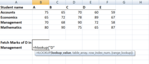
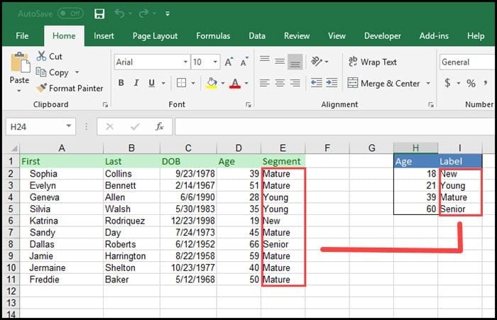
In the formula B15 is the value you want to sum based. Using the same table the marks of students in subject Business Finance are given in sheet 2 as follows. In this MS Excel video tutorial youll learn about using the HLOOKUP function to generate adaptable grades from marks.

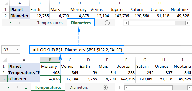
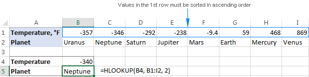
Use HLOOKUP when your comparison values are located in a row across the top of a table of data and you want to look down a specified number of rows. We will use the following formula. To pull out matching data from a different worksheet you specify the sheet name followed by an exclamation mark.

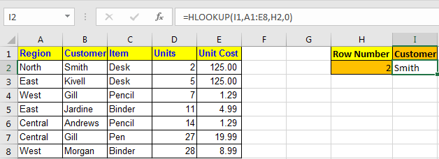
Excel Lookup Multiple Sheets All we need to change is the col_index_number argument like this. We enter the VLOOKUP function in the blank cell where we need to extract the data. Formatting Text.

This method requires a little preparation but in the end you will have a more compact formula to Vlookup in any number of spreadsheets. In simple terms this function takes the users input searches for it in the excel worksheet and returns a matching value related to the same input. This will prompt you to specify the area of the data table.

LOOKUP but this is only included for compatibility with older spreadsheet applications so well concentrate on VLOOKUP and HLOOKUP. Formatting Text. Follow the step-by-step tutorial on how to VLOOKUP for multiple sheets with example and download this Excel workbook to practice along.

Type this formula INDEX D2D10MATCH 1 A2A10G2 B2B10G30 into a blank cell and press Ctrl Shift Enter keys. Use HLOOKUP to sum values based on a specific value.

How To Use The Hlookup Function In Google Sheets Sheetgo Blog